Feature extraction for Vehicle Detection using HOG+

This is how I went about doing the Vehicle Detection project (P5) from Term 1 of the Udacity’s Self Driving Car Nanodegree program. The goals / steps of this project are the following:

• Perform a Histogram of Oriented Gradients (HOG) feature extraction on a labeled training set of images and train a classifier Linear SVM classifier
• Optionally, you can also apply a color transform and append binned color features, as well as histograms of color, to your HOG feature vector.
• Note: for those first two steps don’t forget to normalize your features and randomize a selection for training and testing.
• Implement a sliding-window technique and use your trained classifier to search for vehicles in images.
• Run your pipeline on a video stream (start with the test_video.mp4 and later implement on full project_video.mp4) and create a heat map of recurring detections frame by frame to reject outliers and follow detected vehicles.
• Estimate a bounding box for vehicles detected.

This article will cover the first two steps.

Visualizing the data

The first step always is to see what we’ve got. And here is the data from Udacity. Some examples of cars and non-cars that we’ve are

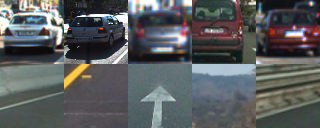
Some things to note here are that each image is a 64x64. And there are about 8k images of each type. Which considering that the background class is pretty much everything other than car, I guess is a pretty small image set.

Image Features

The course suggests to use a combination of multiple image features. Once again we are doing this detection using traditional CV techniques as opposed to using modern CNN architectures like YOLO / SSD.

So we’ve the following image features along with the following parameters for each image features

• Spatial binning (features directly extracted from the image pixels): Color space of the image (commonly used for other features too); Size of the image to be binned
• Color histogram: Number of histogram bins
• Histogram of oriented gradients (HOG): Channel used, Orientations, Pixels per Cells, Cells per block

Choosing the parameters

In terms of choosing the parameters, we’ve two major rationales. One is speed, we don’t want to wait for ages for the classification to happen, and in the best case, we want it to be real time. The other is accuracy. So the parameter decisions is a trade-off between these two attributes.

Visualizing the parameters

Once again the shortcut is to visualize the parameters to get an intuition of how they work.

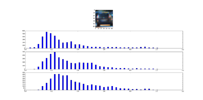
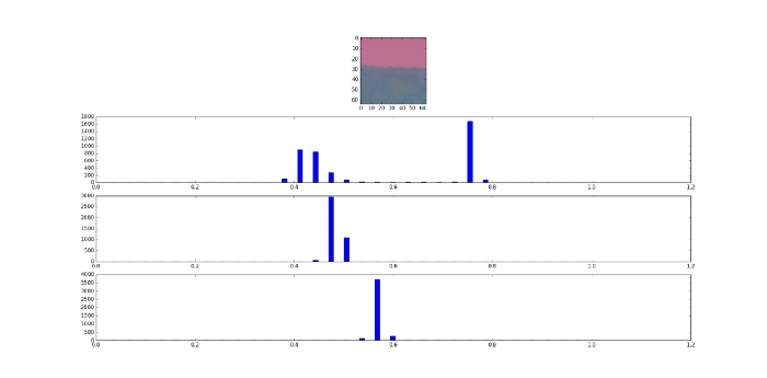
We can see that for the RGB color space, all the 3 channels give us a very different spectrum across the histogram. So this looks good.

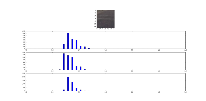
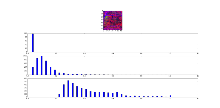
Here, the Y channel gives a good difference, but the Cb and the Cr channels look almost similar. So does not look like a good choice.

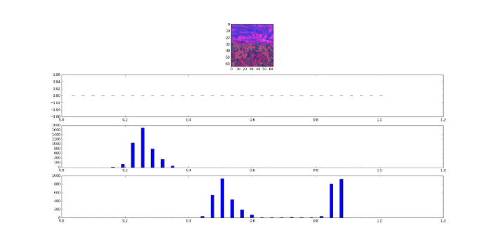
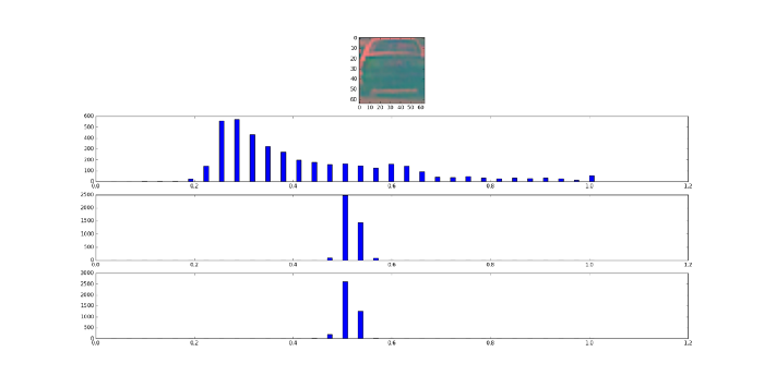
Here, we see a decent difference in S and V channel, but not much in the H channel. So maybe in terms of color histogram, RGB and the S & V channel of HSV are looking good.

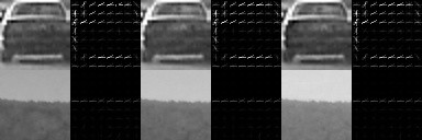
Great! Now let’s visualize the HOG parameters.

The combinations used here are

1. Orientations = 8, Pixel per cell = (8,8), cells per block = 2
2. Orientations = 9, Pixel per cell = (8,8), cells per block = 2
3. Orientations = 8, Pixel per cell = (16,16), cells per block = 2
4. Orientations = 9, Pixel per cell = (16,16), cells per block = 2
5. Orientations = 8, Pixel per cell = (8,8), cells per block = 1
6. Orientations = 9, Pixel per cell = (8,8), cells per block = 1
7. Orientations = 8, Pixel per cell = (16,16), cells per block = 1
8. Orientations = 9, Pixel per cell = (16,16), cells per block = 1

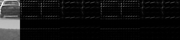
The first option looks great! Nice clear markings for the car image, and a clear difference between the car and non-car image

Now let’s look at the color spaces within HOG

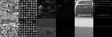
We get almost the same result as we got in the color histogram, which is a great reaffirmation for the data. The YCbCr gives a differential performance only for the Y channel. Whereas all 3 channels in RGB gives us a difference. The Hue in HSV is almost similar, but the S and V show a nice difference.

Training the Classifier

Before we train, we need to ensure that all the features are normalized. WE can use the StandardScaler in sklearn to get this to work easily.

Let’s actually train the SVM and check SVM’s accuracy to see if it corresponds to the data that we’ve got till. In the following experiment, I fixed the hog orientations to 8, hog pixel per cell to be 8 and cells per block to be 2. I’ve also fixed the spatial binning size to be 16x16 and the color histogram bins to be 16. The only variations are the color space.

• Y channel of YCbCr (no spatial binning or color hist): 93.53%
• RGB (all 3)(no spatial binning or color hist): 96.07%
• SV channel of HSV(no spatial binning or color hist): 95.97%
• SV channel of HSV (with spatial binning or color hist): 98.51%
• HSV (all 3)(with spatial binning or color hist): 98.86%
• RGB (all 3)(with spatial binning or color hist): 97.73%

Awesome. So we’ve got our winners. It’s HSV, where the H channel is optional (trading off speed to accuracy). So that covers the feature extraction part of the Vehicle Detection.

As alternatives, you can also look at a standard CNN as a feature extractor.